Identifying tissue domains
Cells are organised into tissues and organs. Spatial gene expression not only allows the identification of cell types in situ, but also allows investigation of how these cells are organised.
SSAM facilitates the identification of “tissue domains”, which are
regions in the tissue exhibiting similar local cell type composition.
This is based on circular window sampling with a defined radius and
step, which is then followed by agglomerative
clustering.
Perform circular window sampling
The first step is to sample cell-type composition in circular sweeping
windows. For this, the size of circular window (radius) and the step
between each sampling (step) has to be defined. The units here are
in um, which is also equivalent to pixels in this example. The following
performs this sampling using a circular window of 100um, with 10um
steps:
analysis.bin_celltypemaps(step=10, radius=100)
Clustering domain signatures
After performing the sampling, we continue with identifying domain
signatures through clustering. This is based on agglomerative clustering
to identify the initial clusters (n_clusters) of windows which
include a minimum number of classified pixels (norm_thres), followed
cluster merging when the correlation between clusters exceeds a
threshold (merge_thres). The merging of clusters can be restricted
to adjacent clusters (merge_remote=FALSE), or not restricted to
spatial proximity (merge_remote=True)
analysis.find_domains(n_clusters=20, merge_remote=True, merge_thres=0.7, norm_thres=1500)
Visualizing identified domains
Once the domains have been indentified, they have to be visualised for evaluation.
from matplotlib.colors import ListedColormap
cmap_jet = plt.get_cmap('jet')
num_domains = np.max(ds.inferred_domains_cells) + 1

fig, axs = plt.subplots(1, num_domains, figsize=(4*num_domains, 4))
for domain_idx in range(num_domains):
    ax = axs[domain_idx]
    plt.sca(ax)
    plt.axis('off')
    cmap = ListedColormap([cmap_jet(lbl_idx / num_domains) if domain_idx == lbl_idx else "#cccccc" for lbl_idx in range(num_domains)])
    ds.plot_domains(rotate=1, cmap=cmap)
plt.tight_layout()
plt.savefig(f'plots/domains_individual')

side by side plot of all tissue domains
Post-processing the identified domains
In certain cases, one may wish to exclude certain domains
(excluded_domain_indices) as they may originate from tissue
artifacts or contain no information. In our case the third domain (0
based index 2) seems to be an artifact and the fourth one contains no
useful information. The First two domains are obviously part of the same
layer and can therefore be merged.
Due to possible imaging artifacts such as tiling, some domains might be
split. While it is still possible to tune the merge_thres in the
clustering step, one can simply perform this as manual post processing.
In the case above, there do not appear to be any domains that require
merging.
Once the domains to be excluded or merged have been determined, they can be excluded and removed(!):
excluded_domain_indices = [2,3,7,10]
merged_domain_indices = [[0,1],[9,11]]
analysis.exclude_and_merge_domains(excluded_domain_indices, merged_domain_indices)
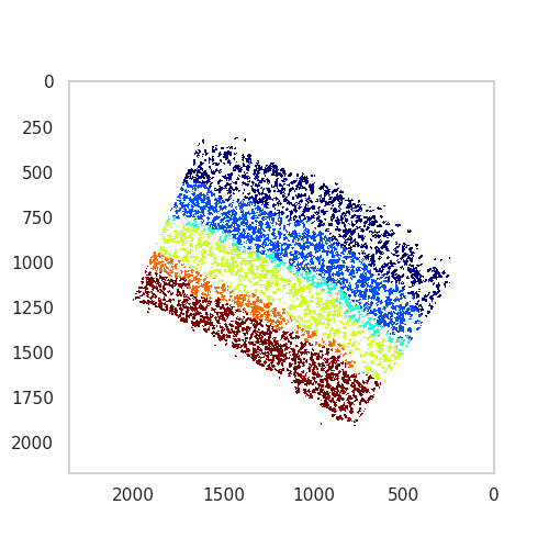
The final plot
The individual domains represent the established neocortex layering patterns found in the mouse brain. We can continue with assigning domain colours, names, and plotting all of the domains together.
plt.figure(figsize=[5, 5])
ds.plot_domains(rotate=1)