SSAM de novo analysis¶

While we believe that the guided mode of SSAM to be able to generate good cell-type maps rapidly, the de novo mode provide much more accurate results.

The steps of the de novo analysis are briefly discussed below, with links to more detailed discussion:

Clustering of expression vectors¶

Once the local maxima have been selected and filtered, we can perform clustering analysis. SSAM supports a number of clustering methods. Here we use the Louvain algorithm using 22 principle components, a resolution of 0.15.

analysis.cluster_vectors(
    min_cluster_size=0,
    pca_dims=22,
    resolution=0.15,
    metric='correlation')

Cluster annotation and diagnostics¶

SSAM provides diagnostic plots which can be used to evaluate the quality of clusters, and facilitates the annotation of clusters.

Visualisng the clusters¶

SSAM supports cluster visualisation via heatmaps, and 2D embedding (t-SNE and UMAP). Here we give an example of the t-SNE plot:

plt.figure(figsize=[5, 5])
ds.plot_tsne(pca_dims=22, metric="correlation", s=5, run_tsne=True)
plt.savefig('images/tsne.png')

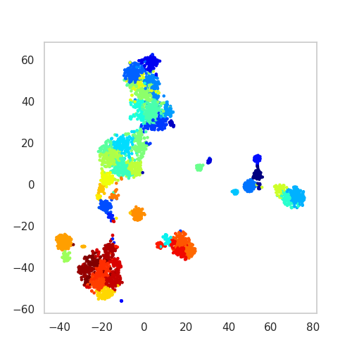
plot of t-SNE embedding of cell types

Cell type map¶

Once the clusters have been evaluated for quality, we can generate the de novo cell-type map. This involves classifying all the pixels in the tissue image based on a correlation threshold. For the de novo application 0.6 was found to perform well:

analysis.map_celltypes()

filter_params = {
    "block_size": 151,
    "method": "mean",
    "mode": "constant",
    "offset": 0.2
    }

analysis.filter_celltypemaps(min_norm="local", filter_params=filter_params, min_r=0.6, fill_blobs=True, min_blob_area=50, output_mask=output_mask)

plt.figure(figsize=[5, 5])
ds.plot_celltypes_map(rotate=1, set_alpha=False)
plt.axis('off')
plt.savefig('images/de_novo.png')

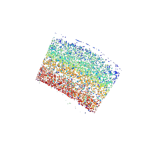
plot of the de novo generated celltype map

We can now use our celltype map to infer a map of tissue domains.