Creating the vector field
After the data has been loaded, SSAM converts the discrete mRNA locations into mRNA desntiy (that can be thought of as continuous “gene expression clouds” over the tissue) through application of Kernel Density Estimation.
KDE
With our SSAMDataset object ds we can now initialize a
SSAMAnalysis object analysis.
analysis = ssam.SSAMAnalysis(
  ds,
  ncores=10, # used for kde step
  save_dir="kde/",
  verbose=True)
And calculate a mRNA density estimate with the run_kde method.
Important considerations here are the kernel
function and the kernel
bandwidth. As default, we recommend using a
Gaussian kernel with a bandwidth of 2.5:
analysis.run_kde(bandwidth=2.5, use_mmap=False)
Masking
If you want to perform the analysis on only a part of your sample you
can use a mask. This can restrict what parts of the image
are used for local maxima sampling (the input_mask), or restrict the
cell-type map generation of SSAM to certain regions (the
output_mask). While this is not required for analysis (infact the
SSAM paper did not apply masks to the osmFISH or MERFISH dataset), here
we define a simply polygon as both the input_mask and
output_mask for the VISp region.
from matplotlib.path import Path
# manual area annotation
xy = np.array([[1535,  90],
               [ 795,  335],
               [ 135,  940],
               [ 835, 1995],
               [1465, 1695],
               [2010, 1215]])

# Extract coordinates from SSAMDataset
x, y = np.meshgrid(np.arange(ds.vf.shape[0]), np.arange(ds.vf.shape[1]))
x, y = x.flatten(), y.flatten()
points = np.vstack((x,y)).T

path = Path(xy)
input_mask = path.contains_points(points)
input_mask = input_mask.reshape((ds.vf.shape[1], ds.vf.shape[0], 1)).swapaxes(0, 1)
output_mask = input_mask
We recommend a visual inspection of the mask to make sure it alignes with the data as you expect it to:
from matplotlib.patches import Polygon
from matplotlib.collections import PatchCollection

patch = Polygon(xy, True)
p = PatchCollection([patch], alpha=0.4)

plt.figure(figsize=[5, 5])
ds.plot_l1norm(rotate=1, cmap="Greys")
plt.gca().add_collection(p)
plt.axis('off')
plt.savefig('images/mask.png')

plot of the mRNA density superimposed with the mask
Local maxima search and normalization
In order to reduce the computational burden, we recommend downsampling the image. While random sampling can be performe, we strongly encourage downsampling via local maxima selection, followed by filtering based of individual and total gene expression.
The local maxima are used to (i) determine the variance stabilisation parameters for the image, and (ii) be used to determine clusters in de novo analysis. In this section, we will use the local maxima for variance stabilisation.
Here we apply the find_localmax function to find the local maxima of
the mRNA density, using a per gene expression threshold of 0.027 and
a total gene expression threshold of 0.2:
analysis.find_localmax(
    search_size=3,
    min_norm=0.2, # the total gene expression threshold
    min_expression=0.027, # the per gene expression threshold
    mask=input_mask
    )
Visualization
After the local maxima have been identified, they can be visualised. In cases when many local maxima orginate from outside the tissue area a k-NN density threshold can be used to filter “stray” local maxima, however in this example we use an input mask so it is not a problem.
plt.figure(figsize=[5, 5])
ds.plot_l1norm(cmap="Greys", rotate=1)
ds.plot_localmax(c="Blue", rotate=1, s=0.1)

patch = Polygon(xy, facecolor="black", edgecolor="red", linewidth=10, ls="-")
p = PatchCollection([patch], alpha=0.4)
plt.gca().add_collection(p)

scalebar = ScaleBar(1, 'um') # 1 pixel = 1um
plt.gca().add_artist(scalebar)
plt.tight_layout()
plt.axis('off')
plt.show()
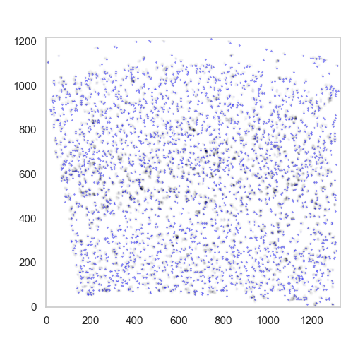
plot found maxima superimposed with the mask
Normalization
Once the local maxima have been identified, we can use them for
calculating the variance stabilisation parameters using sctransform.
If you receive an error here, make sure that you have installed the R
packages in the installation step
This part of the analysis ends with the normalization of the mRNA density and the local-maximum vectors.
analysis.normalize_vectors_sctransform()
Now we are rady to continue with mapping the cell types in guided or de novo mode.